Factor timing – You’re doing it wrong!


6 minute read
The quantitative finance world has recently been transfixed by its version of the East Coast/West Coast feud. But instead of Brooklyn versus Compton rappers, it’s their suburban cousins Greenwich versus Newport Beach arguing over factor timing.
| City | Average household income | Represented by: |
|---|---|---|
| East Coast (New York Area) | ||
| Brooklyn | $51,141 | Notorious B.I.G. (RIP), Sean Combs (Bad Boy) |
| Greenwich | $131,227 | Cliff Asness (AQR) |
| West Coast (Los Angeles Area) | ||
| Compton | $45,676 | N.W.A., Suge Knight (Death Row) |
| Newport Beach | $123,351 | Rob Arnott (Research Affiliates) |
Given that our hubs are London and Denver, we’ve stayed clear of this bi-coastal debate, but clients have asked us for our view. With no axe to grind, we end up somewhere in the middle. Like all investing, if you can time your trades perfectly (or at least better than average) you can beat a mechanical portfolio. There are occasional bubbles (and busts) when a particular factor gets crowded and expensive, and vice versa. Good timing can, by definition, add to returns.
But it’s hard to get this right – and available evidence from ETF-land suggests that the average investor is terrible at factor timing. To show this, we analyse the largest 20 “smart beta” ETFs listed in the US – each have at least $3 billion in assets.
There are three themes that have been popular in smart beta ETFs for several years already – pidends (~$65 billion), low volatility (~$35 billion), and equal weighted (~$16 billion) – so we have a decent history for these styles. Although there are now ETFs available for other factors e.g. value and momentum, those are mostly newer, smaller products.
1.Dividends – the largest ETF for the pidend factor manages ~$17 billion. The ETF has very active creation/redemption (a proxy for net buying/selling respectively) with the number of outstanding units varying considerably over the last few years. The chart below has two lines – the grey line (left axis) shows the number of ETF units outstanding, while the red line (right axis) shows the relative performance of the pidend factor (ratio of ETF total return to S&P 500 total return) over the last three years.
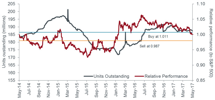
Notably, the total return on the ETF has matched the S&P 500 total return (the relative factor is exactly 1.00 currently) e.g. an investor should have achieved the same return whether picking the ETF or the S&P 500. But the chart above shows that the number of units outstanding typically went up when the pidend factor was outperforming, and went down when the pidend factor was
underperforming.
Looking at only the days that the ETF units were created (net buying) – relative performance averaged 1.011 – i.e. pidend stocks had outperformed the S&P by 1.1%. Similarly for days that ETF units were redeemed (net selling) – relative performance averaged 0.987 – ie pidend stocks had underperformed the S&P 500 by 1.3%. So by actively trading the pidend factor, investors on average lost 2.4% relative to the S&P 500.
This is likely return chasing – when pidend stocks are outperforming, money comes into the factor. Or perhaps money comes in, and pidend stocks outperform – it’s hard to decisively determine the direction of causality. But either way, this example shows that timing the factor is costly to the average smart beta ETF investor.
2.Low Volatility – the largest ETF for the minimum volatility factor has ~$13 billion in assets. Charting the ETF versus relative performance shows a similar result. Although the low volatility factor has done quite well by outperforming the S&P 500 by ~4% over the last three years, the average investor in this ETF has underperformed the S&P 500. On average, creations (net buying) took place at a 1.069 relative performance, and redemption (net selling) took place at a 1.049 relative performance. So investors on average lost 2% relative to the S&P 500 by transacting, and the factor is currently at 1.039 or about 3% below the average entry level of 1.069.
Thus, even in a factor that has clearly outperformed the S&P 500, the average investor is worse off than a passive S&P 500 holder.
We see this effect even in low volatility products targeting international markets. A minimum volatility emerging markets ETF was extremely popular in recent years as investors wanted EM exposure but also low volatility. Consequently this ETF significantly outperformed the broader MSCI EM index and inflows poured in. However, this relative performance has reversed with the low volatility ETF now trailing the basic EM index significantly. Over the past year, it has underperformed by ~16%, missing much of the emerging markets rally.
3.Equal-Weighted – this is the simplest and oldest smart beta factor – equal-weighting an index provides a modest size and value tilt relative to market capitalization weights. Given the strong market rally, equal-weighted has underperformed market-cap by about 3.5% over the past 3 years. The largest ETF in this space manages ~$13 billion. Notably, this has been a stickier product with assets relatively stable. Nevertheless, even in this ETF, the number of units outstanding has often correlated with relative performance as shown in the chart below. The average buy level is about 1% above the average sell level (in relative performance terms).
All the examples above show a consistent result – factor timing is hard and the average investor, at least those using ETFs, tend to get it wrong by piling into factors that are working and vice-versa. Instead, this investor behaviour is often a signal to do the opposite trade – buy after large outflows, and sell after large inflows to a factor ETF.
In the alternative funds that we manage, we typically prefer strategies that instead provide liquidity e.g. buy when others need to sell and vice-versa. Doing this has historically generated alpha over the long-term, avoids crowding, and minimizes transaction cost impact. We look for these flow-driven price pressure trades in both equity and fixed income markets.
Importantly, we are not a factor shop like our East Coast/West Coast brethren – we typically avoid running well-known quant factors. Assets in smart beta ETFs are likely just the tip of the iceberg. There is certainly much more money running similar factor strategies in managed- and internally-run accounts in addition to what is publicly disclosed by ETFs and mutual funds. Thus, we cannot ascertain whether these factors are crowded or not, and we largely sidestep this quant feud by mostly pursuing strategies that are independent to these factors.
These are the views of the author at the time of publication and may differ from the views of other individuals/teams at Janus Henderson Investors. References made to individual securities do not constitute a recommendation to buy, sell or hold any security, investment strategy or market sector, and should not be assumed to be profitable. Janus Henderson Investors, its affiliated advisor, or its employees, may have a position in the securities mentioned.
Past performance does not predict future returns. The value of an investment and the income from it can fall as well as rise and you may not get back the amount originally invested.
The information in this article does not qualify as an investment recommendation.
Marketing Communication.