
Key takeaways:
- The spread between single-stock and index-implied volatility is near historic extremes, meaning index-based ELNs currently offer less income per unit of risk. This pricing signal favors single-name structures in the current environment.
- The ability to pivot between single-name and index-based structures as volatility regimes and correlations shift is an important advantage of an actively managed ELN portfolio.
- True ELN diversification extends beyond the underlying asset to structure type, maturity, observation dates, and counterparties – each an often-overlooked layer for uncovering meaningful value.
The income an equity-linked note (ELN) generates is not arbitrary; it reflects a specific set of market conditions, including implied volatility levels, counterparty pricing dynamics, and the structural supply and demand for certain types of risk. For investors already familiar with ELNs, these forces may be well understood in isolation. But in our experience, they are often underappreciated when it comes to how they interact — and where they create opportunity.
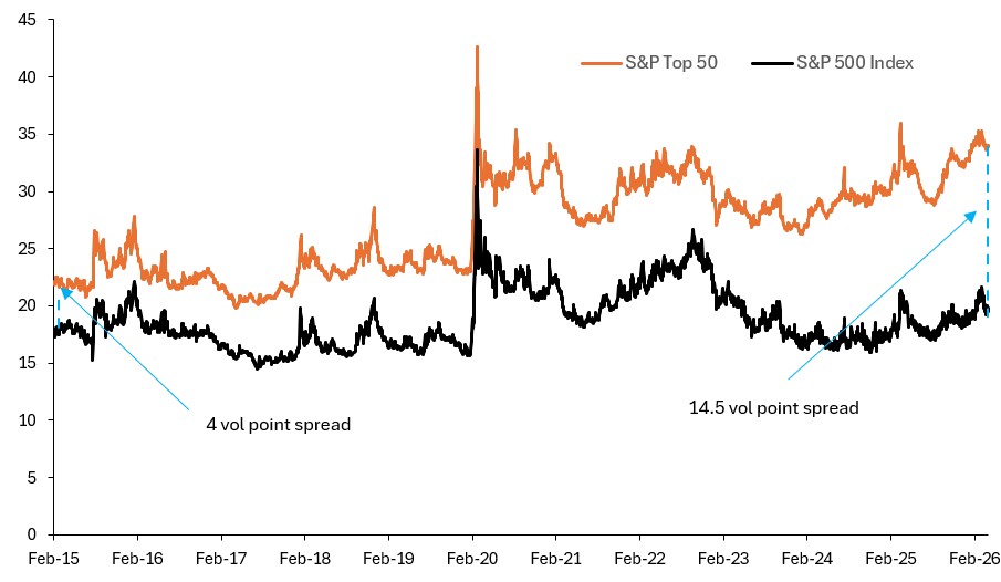
Today, for instance, the gap between single-stock and index volatility is near historic extremes, creating a meaningful difference in the income available depending on which underlying exposure a portfolio uses. That kind of pricing signal matters, and so does the flexibility to act on it.
As the ELN market has grown and more investors gain access through fund structures, we think it is worth examining the variables that drive outcomes — from portfolio construction to pricing inefficiencies — and the considerations that matter most when building a diversified portfolio of these instruments.
Understanding ELNs and the source of income
ELNs are structured products — debt securities whose returns depend on the performance of an underlying asset such as a stock, index, or basket. They embed options that define both the income potential and downside exposure for each note. In practice, similar payoff profiles can also be accessed through derivative contracts, such as swaps, which replicate ELN outcomes without taking issuer credit risk.
At their core, ELNs generate income by compensating investors for bearing a defined risk. This can be thought of as an insurance-style arrangement: The investor receives a coupon — the “premium” — in exchange for absorbing the possibility that an underlying stock or index falls by a specified amount. If that doesn’t happen, the investor earns income and receives principal back. If it does, a capital loss results.
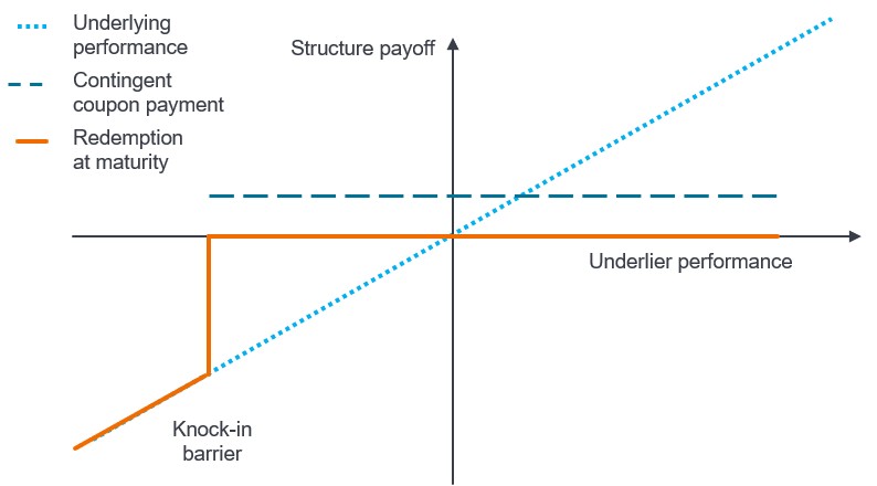
One of the most common income-focused structures is the autocallable. These instruments typically offer elevated coupons but may automatically redeem early if the underlying asset trades above a predefined level on observation dates. Its value lies in offering yield and potential downside buffers in range-bound or moderately positive markets. While this structure can enhance income, it also has the potential for capital loss if the underlying declines beyond a specified barrier at the maturity date, including mark-to-market losses on the way to that barrier price.
Exhibit 1: Autocallable redemption profile at maturity
Source: Janus Henderson Investors.
What makes ELNs distinctive is that this risk is highly customizable. The underlying exposure, level of downside risk mitigation, observation frequency, and maturity can all be adjusted. But the fundamental tradeoff remains: A higher coupon always reflects more risk, whether a higher likelihood of loss, a greater magnitude of loss, or both.
One nuance worth emphasizing: Barrier protection reduces the frequency of losses, but it does not reduce their severity when they do occur. If an underlying asset falls far enough to breach the barrier, the loss can be substantial. Understanding that distinction is essential to building a portfolio that balances income generation with risk management.
Diversification beyond the underlying asset
When investors think about diversification in the context of ELNs, the first instinct is often to consider the underlying stocks or indices. That matters, but there are other layers of diversification to consider.
At the structure level, different note types carry distinct risk and return profiles. Autocallables, introduced earlier, tend to offer higher coupons but come with path dependency: Their performance depends on where the underlying trades at specific observation dates over the lifetime of the structure.
Stability notes, by contrast, provide lower yields but insure against a specific and remote risk: an extreme single-day move lower in the underlying. Because their barriers reset daily relative to the prior close, stability notes tend to carry very little market beta in normal conditions.
Exhibit 2: Stability note redemption profile at maturity
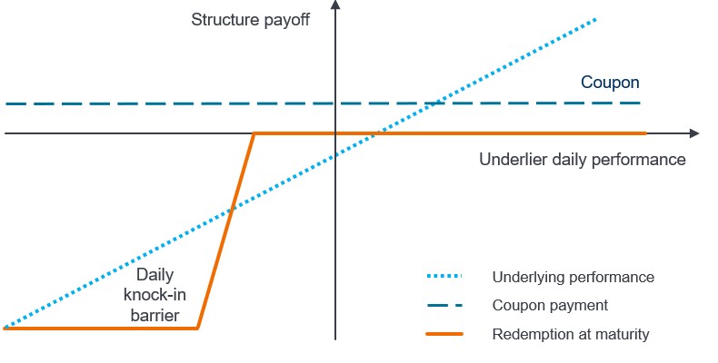
Source: Janus Henderson Investors. Note: Typical daily return of the reference asset/index needed for a stability note to begin suffering principal loss. Examples for illustrative purposes only and do not represent the returns of any particular investment.
We view these two structures as natural complements. When markets trend steadily lower, stability note pricing remains far more stable than autocallable pricing, which can help anchor a portfolio’s value.
Stability notes also benefit from an interesting structural dynamic. Banks are, in some cases, regulatory-driven sellers of extreme gap risk — they are required to stress-test for severe single-day moves, and selling these notes allows them to hedge some of that exposure. That structural supply can, in certain environments, make stability note pricing attractive relative to the remote nature of the risk being insured.
Looking at 100 years of daily returns for a major equity index, only one trading day out of roughly 25,000 — Black Monday in 1987 — produced a single-day decline exceeding 15%, a typical barrier level for these notes (see Exhibit 3). That does not mean it cannot happen again, but it illustrates the type of tail risk being insured.
Exhibit 3: Worst single-day S&P 500® Index returns in last 100 years

Source: Bloomberg, as of 31 January 2026. Past performance does not predict future returns.
Beyond structure type, a well-constructed portfolio should also diversify across maturities, observation dates, and counterparties. Laddering maturities and staggering coupon observation dates helps smooth the income stream so the portfolio may not be overly reliant on market conditions at any single point in time. Sourcing from multiple counterparties – and where appropriate, accessing exposures through swaps – helps reduce credit risk and can itself be a source of value.
The same structure can be priced quite differently depending on how it fits a given counterparty’s book. That dispersion in pricing is, in our view, one of the more underappreciated inefficiencies in this market.
Reading the market’s pricing signals
We believe one of the most valuable aspects of active management in this space is the ability to read what the market is pricing and position accordingly. Suffice to say, predicting the future is not possible. But evaluating current pricing and assessing what is already built into the price of future volatility can meaningfully improve outcomes.
Consider the current environment. The level of volatility priced into broad index options versus single-stock options reflects an unusually wide spread by historical standards (see Exhibit 4). There is higher volatility priced into single stocks (orange line) compared to the volatility priced in for index options (black line).
Put differently, the implied correlation between individual stocks — the correlation priced into an index or basket derivative — is near historically low levels, and not far from zero. This has been driven in part by the fact that realized correlations have been low. But when you buy an ELN or trade an option, you are effectively locking in the price of that future volatility.
Exhibit 4: S&P Top 50 vs. S&P 500 Index implied volatility
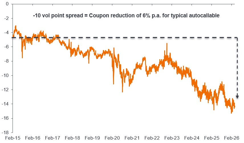
Source: Janus Henderson Investors, Bloomberg, as of 27 April 2026. S&P Top 50 takes the cross-sectional weighted average volatilities of the top 50 S&P 500 Index constituents. Implied volatilities are 2-year at-the-money. Note: *Typical autocallable is defined as a 2yr structure with S&P 500 underlier, 70% coupon /maturity barrier and coupon semi-annual observations. 6% is the difference in annualized coupon between an autocallable on the S&P 500 and the same structure but with the S&P 500 volatility increased by 10 volatility points.
The practical impact is significant: On a standard two-year autocallable with a 70% barrier on a major equity index, a 10-volatility-point shift in implied volatility — roughly the magnitude of the spread’s movement over the past decade — translates to approximately a six percentage-point difference in annualized coupon. Because single-stock implied volatility is elevated relative to index volatility today, an index-based autocallable currently pays meaningfully less income per unit of risk than it did when that spread was narrower.
For us, this creates a clear signal: In the current environment, single-name autocallables may offer a more attractive income-to-risk tradeoff than index-based structures. If the low-correlation environment persists, both approaches perform similarly. But if correlations revert — whether through rising index volatility or falling single-stock volatility — single-name positioning would tend to be better compensated.
The key is having the flexibility to pivot. If correlations spike, a portfolio can shift toward index-based structures to capture that opportunity.
Always on, not set and forget
Building a portfolio of ELNs is not a static exercise. Market conditions shift. Volatility regimes change. Counterparty pricing evolves. The structures that offered the best risk-adjusted income six months ago may not be the most attractive today.
The value of active management comes from a continuous process: reading pricing signals, diversifying at every level of the portfolio, and maintaining the flexibility to adapt.
That flexibility extends to risk management as well. In certain environments, it may be prudent to hedge tail risks at the portfolio level — through index options, for example — even though doing so comes at some cost to income. Hedging will not always be warranted, but having the ability to deploy it when market conditions call for it is an important part of the toolkit.
The goal is straightforward: to seek to deliver on income targets while keeping portfolio risk levels as low as possible. Achieving that goal requires discipline, expertise, and the ability to go wherever the market presents the best opportunity.
An autocallable note is a note that may be automatically redeemed if the underlying asset rises above a preset level.
Barrier is a price threshold that affects coupon payments or principal protection.
Beta measures the volatility of a security or portfolio relative to an index. Less than one means lower volatility than the index; more than one means greater volatility.
Correlation measures the degree to which two variables move in relation to each other. A value of 1.0 implies movement in parallel, -1.0 implies movement in opposite directions, and 0.0 implies no relationship.
Gap risk is the risk of a sudden, material overnight market decline that cannot be readily hedged by banks.
A stability note is a note that pays income unless the underlying experiences a one-day drop beyond a set limit.
Volatility measures risk using the dispersion of returns for a given investment.
IMPORTANT INFORMATION
Actively managed portfolios may fail to produce the intended results. No investment strategy can ensure a profit or eliminate the risk of loss.
Autocallable instruments limit upside because payouts may cease once an autocall occurs, resulting in missed future income opportunities and reinvestment at potentially less favorable levels. Barrier events can suspend income or reduce principal if predefined levels are breached. Depending on the terms, investors may receive no further coupons and may experience partial or total loss of principal following adverse market movements.
Diversification neither assures a profit nor eliminates the risk of experiencing investment losses.
Equity linked notes (ELNs) are structured obligations whose value is derived from an equity or equity index. ELNs may be difficult to value or sell, may lack active secondary markets, and may not fully participate in equity market gains. Because ELNs are unsecured obligations of issuing banks or broker dealers, investors are exposed to issuer credit risk and may experience losses if the issuer becomes unable or unwilling to meet its obligations. Many ELNs contain call features that can terminate future coupon payments and require reinvestment at less favorable terms.
Equity securities are subject to risks including market risk. Returns will fluctuate in response to issuer, political and economic developments.
Stability instruments rely on formulas that adjust payouts when daily market movements breach defined stability levels, which can lead to reduced income or early redemption at values below the amount invested. These instruments do not guarantee principal and may expose investors to amplified losses if leveraged components are triggered. Payoff structures may limit participation in market gains while increasing sensitivity to significant drawdowns.
Swap agreements are derivative contracts that provide synthetic exposure to a reference asset or index and may introduce counterparty default risk, valuation uncertainty, and leverage effects. Returns may differ from the reference exposure due to fees, collateral requirements, or imperfect correlation. Swap exposures may be less liquid or more volatile during periods of market stress.